Essentially, all models are wrong, but some are useful.
- George Box
In its refunding policies one large issuer (and my banking friends know…) has indicated that it wants banks trying to get refunding business to provide the “estimated value of the advance refunding option (incremental to the value of the call/current refunding option).” This leaves a lot of room for interpretation and frankly, leaves many scratching their head. In this article we try to provide some clarity. There are 3 things that must necessarily impact any estimate of the “value of the advance refunding option.”
- Refunding Policy
The issuer in question uses “85% refunding efficiency” as the exercise heuristic that indicates a time to refund. If they used 75% or 95% (and why not?) then these changes would necessary lead to different option values. Though some may try to argue otherwise, this is simple financial reality – the decision trigger upon which an option is exercised MUST impact the value of the option. How could it not? Fortunately, there’s good research on which refunding policies work and which don’t both historically back-tested and on a prospective basis using a real-world market model. For the Cliff notes I just wrote an article on the one that works best in both environments. And its simple too - fancy models need not apply.
- Yield Curve / Rate View
The hard thing about refunding timing is that it necessarily involves an interest rate call. The muni market is not and, unless tax law changes, never will approach the nice, antiseptic, no-arbitrage market required by standard option models. Issuers have real skin in the game, can’t hedge their positions, and as such fall into the uncomfortable world of rate risk management. So no refunding decision criteria can fully divorce itself from at least an implied rate view. And researches from the SanFran Fed just recently cautioned against using market implied measures (read “forward rates”) for policy purposes.
- Muni / taxable view
But how are these two interrelated but very different markets modeled? What factors drive their variability and what is the correlation between them? Unfortunately there are no observable options that trade where we could see the market implied correlation between munis and US Treasuries. This is another reason why a real-world model is necessary. But any model that credibly handles this multi-market modeling should fully describe how this bridge is traversed; it’s both treacherous and fundamental to the analysis.
Advance Refunding “Option” – Some Real-World Results
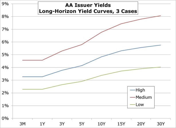
Enough gum flapping. Let’s look at some numbers. We created simulated yield curves using our MarketMaker model. Although we created 5 correlated market simulations simultaneously (AAA, AA, A, BBB tax-exempt and SLGS), we assume the issuer is AA and use SLGS markets for the escrow; in the end we only use 2 of the 5. We included 25 years of yield data as input to the variability in the model. Given the eight tenors per market this is a 40 factor model perfectly reproducing the inter- and intra-market correlations/covariance of all 40 tenors.
Now let's look at two bonds. They both are 5% coupons maturing in 25 years, callable in 5 (5% 25NC5), but one is advance refundable and one is not. Given my comment above about the importance of a market view we examine these two bonds under three different expected yield curve scenarios, ‘Low’,’Medium’, and ‘High.’
Let’s start by looking at some simple present value savings thresholds. Using first generation simulated refunding savings, we can compare the expected PV (EPV) savings from the advance refundable bond and non-advance refundable bond at various present value savings thresholds for our refunding policy.1 Here we use the Medium rate case.
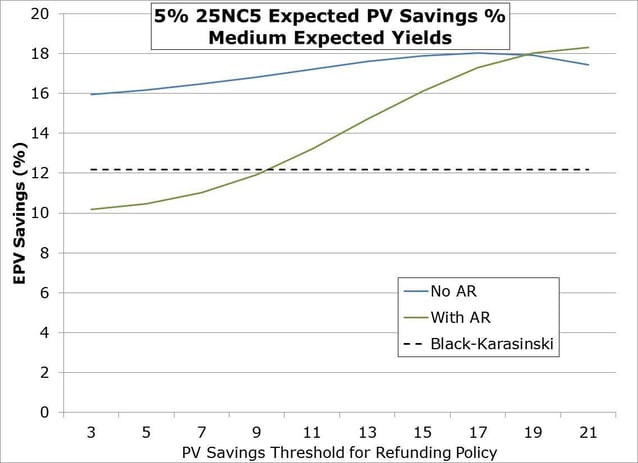
Now these bonds have some real juice since there’s 20 years of 5% par callability happening; the issuer doesn’t maximize EPV savings using low pv savings thresholds. But the important thing to look at is the difference between the lines. The higher EPV savings is generally coming from the non-advance refundable bond, implying a negative value to advance refundability – using these refunding policies and under this Medium yield curve view. What’s happening? Well on average within the model the issuer is generally better off waiting to the call if the refunding timing criterion employed is a simple PV savings threshold. These numbers bear that out. Note we’ve also included a Black-Karasinski bond option value using 15% volatility (as noted in this issuer’s policy guidelines for the refunding efficiency calculation) which is insensitive to PV savings threshold.
See that at about the 19% PV savings threshold the lines cross, and the advance refundable bond EPV savings begins to go higher than the non-AR bond. This tells us the policy obviously matters, as I posited earlier.
In the low yield case we'll get the same sort of relationship since waiting when yields stay low, on average, will handicap advance refundability. So let's look at the high yield case.
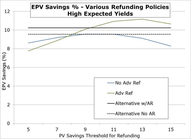
With high yields expected on average, as one would expect EPV savings for the non-advance refundable bond (blue line) is having a larger negative impact particular when looking at the higher PV savings thresholds. The advance refundable bond (green line) tends to dominate on any refunding policy over about 7% PV savings. Here we also show EPV savings calculations for the Alternative Policy (a two pronged policy, see here for details) to see how it compares. It is known that relatively speaking, the Alternative policy will fare less well in fast rising yield environments. But here we see that there’s consistent performance for both AR (solid black) and non-AR (black dotted) bonds, with the AR bond showing slightly more EPV saving.
This made me wonder about the performance of the Alternative policy for these two bonds in all three yield environments.
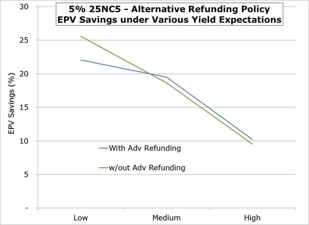
As we’d expect the highest EPV savings corresponds to the lowest expected yield environments and vice versa. But the comparison of the AR and non-AR values is the punch line. In medium and high expected yield environments, the AR bond EPV savings (blue line) inches out the non-AR bond EPV savings (in green). But in the low expected rate environment the fact that the non-AR bond forces the issuer to wait to do a current refunding doesn’t hurt EPV savings. In fact it helps, implying again that the ARO value is negative in that case.
But that leads us to the semantic and perhaps existential question, "Can an option have negative value?" In a traditional financial economic sense the answer is clearly no. But once again, we’re not in Kansas any more. This is muniland’s veritable Oz. Here the answer is, “It depends.”
1 For details about the computatoin of expected pv savings see Aalyzing Municipal Refundings Using a Real-World Market Model.
Comments