"Those who trust to chance must abide by the results of chance." - Calvin Coolidge
"The problem is not their estimates, it's the range of potential error in those estimates." - Alan Greenspan
Despite all behavioral finance has revealed about over-confidence and specifically, the overuse of historic averages in finance, one pervasive legacy of the ubiquitous spreadsheet is a stubborn reliance on static numeric assumptions for market risk factors - “Let’s just use 3% for SIFMA to run that debt service schedule and do the analysis.” It’s such a common modus operandi that it happens often without a second thought. The reality is that keeping variability in the analysis of market variables (where it belongs) is more conceptually challenging, but infinitely better at providing meaningful information to issuers; the right tools can offer critical intuition.
This post describes four risks a skilled modeler with well-designed Monte Carlo tools can explore when looking at tax-exempt variable rate debt (VRDBs).
1. Interest rates
Perhaps less so today, but the primary risk factor people evaluate
in VRDBs is what might happen to the economy and its impact on the demand for short-term money. Of course, what happens at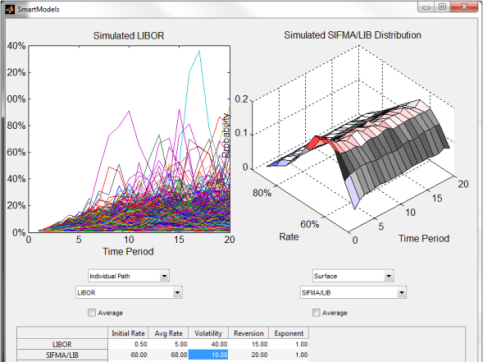 the front of the yield curve is almost entirely driven by those dwellers of the Temple at the Fed. When evaluating tax-exempt VRDBs it makes the most modeling sense (for reasons explained in far more detail in this paper) to first capture some primary benchmark of overall interest rates. Usually, we start with LIBOR.
Note that for each period in the analysis, we’re creating an entire distribution of rates from the simulations as shown in the left LIBOR graph above. We use a straightforward but powerful interest rate model described in detail here.
2. Tax-exempt / Taxable Ratio (SIFMA / LIBOR)
If US tax law changes in a way that diminishes the benefit of tax-exempt income to investors, issuers will immediately face higher costs of borrowing. For this reason, the risk that tax-exempt yields trade closer to taxable ones is actually a component of the variable rate bonds themselves. NOTA BENE: this has nothing to do with whether or not there’s a swap hedging the interest rate risk in the bonds (the press has a hard time with this one).
The essential feature to capture of this basis risk is its inverse relationship with rates. When rates are high, ratios are low and vice versa. This has been a persistent feature of these markets through boom and bust and ignoring it, frankly can lead to expensive mistakes detailed here.
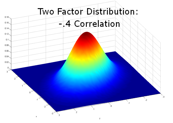
This means the Monte Carlo model needs to have a correlated, multi-factor component. Many are familiar with the most famous distribution (Gaussian or Normal) in one dimension: in this case we need 2 per the image below.
3. Credit support costs
Liquidity support behind VRDBs is no longer a slam dunk. It’s now a much more significant component of cost. In fact, with SIFMA where it is currently, support costs today are generally greater than the interest rate itself! That said these costs are fixed only through the next renewal date. What assumption does an issuer make after that?
A well-designed Monte Carlo simulator allows the user to model the potential changes in credit support costs and add them to the interest rate and basis risks described above.
4. Trading spreads
Much of the joy in public finance lies in the 50,000+ issuer community and its attendant variety. VRDBs are issued by different credits in different states with different tax regimes backed by different banks. As much as SIFMA offers the benchmark against which most variable rate programs are compared, there will undoubtedly be noise around that benchmark, and sometimes that noise is worth trying to understand.
A flexible Monte Carlo rig should provide the user with the ability to model trading spreads, both in expected level and volatility.
5. Converting the VRDBs to Fixed
One plausible “worst case” (one of the three key questions every CFO must ask) might occur if there’s no l the providers with reasonable prices and terms go hiding. In that case, the multi-modal features of the bonds may kick in and the issuer faces a fixed rate remarketing. But what might the market look like then?
With a powerful, generalized simulation framework, the analyst can simulate a long term rate factor, either as part of a complete yield curve simulation or as a separate factor correlated to short term rates. The payments on the bonds then “flip” from the floating index to a (likely higher) fixed rate at the expiration of the letter/line of credit. It’s important to note that the fixed rates are simulated as well, so it’s not just a single fixed rate assumption on the remarketing date, but an entire range of possibilities. This is consistent with the uncertainty associated with that future unknown rate environment.
There you have it. If you need help setting up a model to capture these risks, let us know.
Comments